Usage¶

Authors: Judith Korth and Hannu Parviainen Edited: 4 March 2025

[1]:

%matplotlib inline

[2]:

import matplotlib.pyplot as plt

from numpy import pi
from cheopslcs import LCSim

Simulator setup¶

The light curve simulation is done using cheopslcs.LCSim class, which is initialised by giving the observing window width in hours, exposure time in seconds, and the white noise standard deviation. Optionally, we can also give the limb darkening model used by the transit model (one of: constant, linear, quadratic, nonlinear, general, power-2, and power-2-pm, see the PyTransit documentation for details).

[3]:

lcs = LCSim(window_width=5.0, exp_time=60, white_noise=1e-4)

How to simulate a transit¶

After the simulator has been set up, we can create light curves by calling the simulator as a function. A simple transit can be created by giving the

planet-star radius ratio,
zero epoch,
orbital period in days,
semi-major axis divided by the stellar radius,
impact parameter, and
limb darkening coefficients specific to the used limb-darkening model

as arguments, and the call will return two NumPy arrays containing mid-exposure times and fluxes.

[4]:

time, flux = lcs(radius_ratio=0.1, zero_epoch=0.0, period=2.0,
                 scaled_semi_major_axis=8.0, impact_parameter=0.1,
                limb_darkening=[0.2, 0.3])

fig, ax = plt.subplots(1, 1, figsize=(10,4), constrained_layout=True)
ax.plot(time, flux, '.')
plt.setp(ax, xlabel='Time [d]', ylabel='Flux');

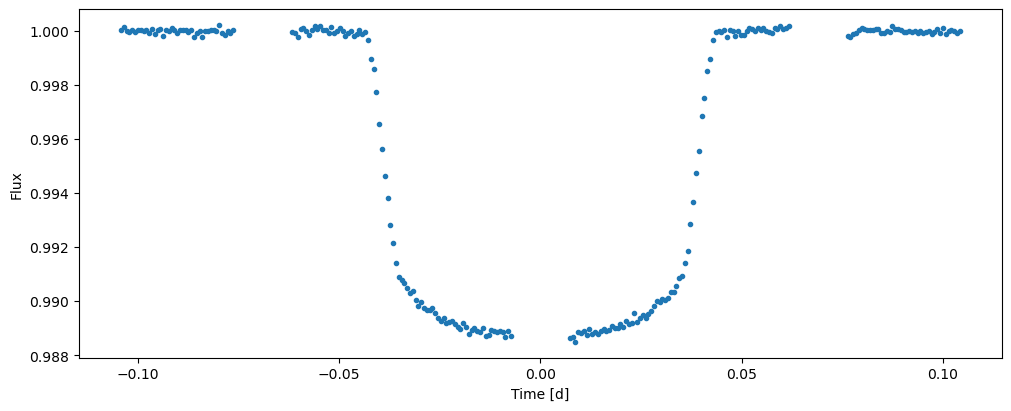
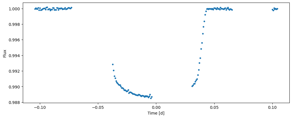
The resulting light curve contains gaps with a period of CHEOPS’s rotation period of 99 minutes. The fractional width and phase of the gaps can be changed with the efficiency and eff_phase arguments. Both efficiency and eff_phase range from 0 to 1; efficiency has a default value of 0.8, and eff_phase defaults to 0.0.

[5]:

time, flux = lcs(radius_ratio=0.1, zero_epoch=0.0, period=2.0,
                 scaled_semi_major_axis=8.0, impact_parameter=0.1,
                efficiency=0.5, eff_phase=0.2,
                limb_darkening=[0.2, 0.3])

fig, ax = plt.subplots(1, 1, figsize=(10,4), constrained_layout=True)
ax.plot(time, flux, '.')
plt.setp(ax, xlabel='Time [d]', ylabel='Flux');

How to simulate a full phase curve¶

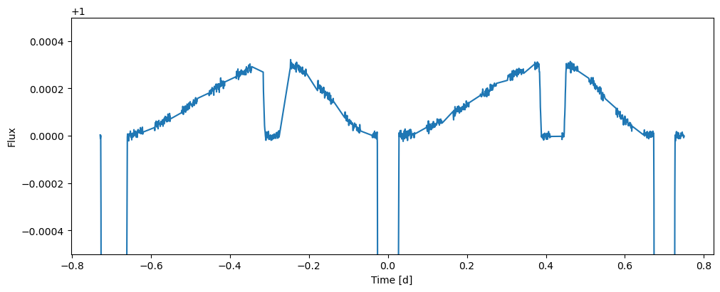
A phase curve with a secondary eclipse can be simulated by giving the simulator a non-zero geometric_albedo argument. Let’s create a long observation of 1.5 days with observing efficiency of 0.6, and also set a non-zero orbital eccentricity and argument_of_periastron to create a more interesting light curve (both eccentricity and argument of periastron can be set for simple transit simulations too, but their effect is very small).

[6]:

lcs = LCSim(window_width=24*1.5, exp_time=60, white_noise=1e-5)

time, flux = lcs(radius_ratio=0.1, zero_epoch=0.0, period=0.7,
                 scaled_semi_major_axis=4.0, impact_parameter=0.1,
                 eccentricity=0.2, argument_of_periastron=0.23*pi,
                 geometric_albedo=0.5, limb_darkening=[0.2, 0.3],
                 efficiency=0.6, eff_phase=0.2)

fig, ax = plt.subplots(1, 1, figsize=(10,4), constrained_layout=True)
ax.plot(time, flux, '-')
plt.setp(ax, ylim=(0.9995, 1.0005), xlabel='Time [d]', ylabel='Flux');